 Physics
📄 Print pdf
00971504825082
Gauss's law and electric field
Electric Field
It is a region surrounding a charge where the effects of electric force appear. It represents the resultant electric force acting on a charge divided by the charge.
The electric field is a vector quantity with magnitude and direction.
\[\vec E=\frac{\vec F_e}{q}= \frac{\frac{K.Q.q}{r^2}}{q}=\frac{K.Q}{r^2}\]
There are two methods to determine direction:
First Method: Place a test charge at the point where direction needs to be determined. According to vector rules, the product of a number and a vector
If a positive test charge is placed, the field direction is the same as the force direction. If the test charge is negative, the field direction is opposite to the electric force direction.

Second Method: By drawing field lines for a positive charge and a negative charge
Field lines for a positive charge emerge from the charge
Field lines for a negative charge converge toward the charge
1

One of the following measurement units is equivalent to the electric field measurement unit
 Click here to show solution method
Choose the correct answer

2
An electric field with intensity \[\vec E=3×10^2\frac {N}{C}\]
An electron is placed inside the field
The electric force acting on the electron equals
\[q_e=1.6 ×10^{-19}C\]
Click here to show solution method
Choose the correct answer
Electric Field Mapping
Properties of Electric Field Lines

They are imaginary lines that emerge from positive charges and converge into negative charges
The density of field lines is directly proportional to the magnitude of the electric charge
The field direction at any point is tangent to the field line at that point
Electric field lines do not intersect
There are two types of electric fields
Uniform field: A field with constant magnitude and direction at all points, its lines are straight and parallel
Non-uniform field: A field with non-constant magnitude or direction or both
Electric Field Due to Point Charges
We previously found that the magnitude of the electric field for a point charge is given by the relation \[\vec E=\frac {\vec F_e}{q}=\frac {K.Q}{r^2}\]
Each point charge generates an electric field around it
If we have more than one charge, each charge generates a field with magnitude and direction
Solved Example

Two point charges
\[q_1 = -6 \;\;𝜇c \;\;\;\;\;\;\;\; q_2 = 4 \;\;𝜇c\]The first charge is placed at the origin
and the second charge is placed at position \[X=5\;\;cm\]Calculate the electric field at position \[X=8\;\;cm\]
Solution
\[E_1=K.\frac {q_1}{r_1^2}=8.99×10^9×\frac {6×10^{-6}}{0.08^2}=8.43×10^6\;\; N/c\] to the left
\[E_2=K.\frac {q_2}{r_2^2}=8.99×10^9×\frac {4×10^{-6}}{0.03^2}=39.95×10^6\;\; N/c\] to the right
\[E_{net}=E_2-E_1=39.95×10^6-8.43×10^6=31.52×10^6\]to the right
Solved Example

Two point charges
\[q_1 = -3 \;\;nc \;\;\;\;\;\;\;\; q_2 = 5 \;\;nc\]placed on triangle vertices as shown in the figure
Calculate the electric field at position
\[A\]
Solution
\[E_1=K.\frac {q_1}{r_1^2}=8.99×10^9×\frac {3×10^{-9}}{0.03^2}=29.9×10^3\;\; N/c\] to the left
\[E_2=K.\frac {q_2}{r_2^2}=8.99×10^9×\frac {5×10^{-9}}{0.04^2}=28.1×10^3\;\; N/c\] downward
\[E_{net}=\sqrt {E_2^2+E_1^2}=\sqrt {(29.9×10^3)^2+(28.1×10^3)^2}=41.1×10^3\;\;N/C\]Direction \[\theta=tan^{-1}\frac{E_2}{E_1}=tan^{-1}(\frac{28.1×10^3}{29.9×10^3})=43.2.2^0\]

(Self-Reading) Electric Field of a Dipole

Dipole: A charged object with two equal and opposite charges.
 When calculating the electric field of a dipole due to two opposite charges,
The field due to each charge is calculated, and vector addition is performed according to vector rules.
Solved Example
Calculate the electric field of a dipole along its axis at a point a distance
(X) from the center of the dipole.
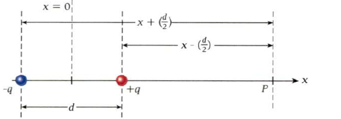
The point is subject to two fields: from the positive charge
\[E_1=\frac{1}{4𝜋𝜀_0}\frac{q}{(X-\frac{1}{2}d)^2}\] (direction to the right)
and from the negative charge
\[E_2=\frac{1}{4𝜋𝜀_0}\frac{q}{(X+\frac{1}{2}d)^2}\] (direction to the left)
The resultant field is \[E_{net}=E_1-E_2\]
\[E_1>E_2\]
\[E_{net}=\frac{1}{4𝜋𝜀_0}\frac{q}{(X-\frac{1}{2}d)^2}-\frac{1}{4𝜋𝜀_0}\frac{q}{(X+\frac{1}{2}d)^2}\]
Direction to the right
Factoring out \[\frac{q}{4𝜋𝜀_0X^2}\]
The equation becomes \[E_{net}=\frac{q}{4𝜋𝜀_0X^2}\left[\frac{1}{(1-\frac{d}{2X})^2}-\frac{1}{(1+\frac{d}{2X})^2}\right]\] Combining denominators \[E_{net}=\frac{q}{4𝜋𝜀_0X^2}\left[\frac{(1+\frac{d}{2X})^2-(1-\frac{d}{2X})^2}{(1-\frac{d}{2X})^2(1+\frac{d}{2X})^2}\right]\]
\[E_{net}=\frac{q}{4𝜋𝜀_0X^2}\left[\frac{(1+\frac{d}{X}+\frac{d^2}{4X^2})-(1-\frac{d}{X}+\frac{d^2}{4X^2})}{(1-\frac{d}{2X})^2(1+\frac{d}{2X})^2}\right]\]
\[E_{net}=\frac{q}{4𝜋𝜀_0X^2}\left[\frac{(1+\frac{d}{X}+\frac{d^2}{4X^2}-1+\frac{d}{X}-\frac{d^2}{4X^2})}{(1-\frac{d}{2X})^2(1+\frac{d}{2X})^2}\right]\]
If \(X \gg d\)
\[\frac{d}{2X} \approx 0\]\[E_{net}=\frac{2dq}{4𝜋𝜀_0X^3}=\frac{dq}{2𝜋𝜀_0X^3}=\frac{2kdq}{X^3}\]
\[P=q.d\] is called the dipole moment, a vector quantity with direction from the negative to the positive charge, opposite to the electric field.

The field can be written as \[E_{net}=\frac{2p}{4𝜋𝜀_0X^3}=\frac{p}{2𝜋𝜀_0X^3}=\frac{2kp}{X^3}\]
Solved Example
Calculate the electric field of a dipole at a point on the perpendicular bisector, a distance
(y) from the center of the dipole.

The point is subject to two fields \[E_1,E_2\]. When resolving each field into components, symmetry shows that
\[𝐸_{1y} = {𝐸_2y}\] and their resultant is zero.
From the figure \[r=\sqrt{(\frac{d}{2})^2+y^2}, \cos 𝜃= \frac{\frac{d}{2}}{r}\]
\[E_{1X}=E_1 \cos 𝜃=\frac{k q}{r^2} \cdot \frac{\frac{d}{2}}{r}=\frac{k q}{(\frac{d}{2})^2+y^2} \cdot \frac{\frac{d}{2}}{\sqrt{(\frac{d}{2})^2+y^2}}\]
\[𝐸_{1x} =\frac{k q d}{2[{(\frac{d}{2})^2+y^2}]^{3/2}}\]
\[E_{2X}=E_2 \cos 𝜃=\frac{k q}{r^2} \cdot \frac{\frac{d}{2}}{r}=\frac{k q}{(\frac{d}{2})^2+y^2} \cdot \frac{\frac{d}{2}}{\sqrt{(\frac{d}{2})^2+y^2}}\]
\[𝐸_{2x} =\frac{k q d}{2[{(\frac{d}{2})^2+y^2}]^{3/2}}\]
\[E_{net}=𝐸_{1x}+𝐸_{2x}=\frac{k q d}{2[{(\frac{d}{2})^2+y^2}]^{3/2}}+\frac{k q d}{2[{(\frac{d}{2})^2+y^2}]^{3/2}}\]
\[E_{net}= -\frac{k q d}{[{(\frac{d}{2})^2+y^2}]^{3/2}}\]
The negative sign indicates the direction is along the negative horizontal axis.
If \(y \gg d\)
\[\frac{d}{2} \approx 0\]
\[E_{net}= -\frac{k q d}{y^3} \]
General Charge Distributions
For a very large number of charges, calculating the resultant field using the previous method is impractical. Instead, integration is used, provided the charges are uniformly distributed.
Take a small part of the object's charge
\[dq\]
calculate its field, then integrate over the entire object.
The problem arises if the charge is distributed along a line, over a surface, or within a volume.
Along a line:
\[𝑑𝑞=λ𝑑𝑥\]
Over a surface:
\[𝑑𝑞=σ𝑑A\]
Within a volume:
\[𝑑𝑞=𝜌𝑑V\]
(Advanced) Solved Example
A finite-length wire is uniformly charged as shown below. Calculate the magnitude and direction of the field at a point along the perpendicular bisector of the wire.

Take a small charge
\[dq\] and calculate its field, then integrate over the entire wire.
Considering half the wire, symmetry shows that
\[E_1X=E_2X\]
They cancel each other out, so the resultant is zero.
The vertical components from each half are equal in magnitude and direction.
\[ d𝐸_1Y =d 𝐸_1 \cos 𝜃 , d𝐸_2Y =d 𝐸_2 \cos 𝜃\]
To calculate the field, compute it for half the wire and double the result.
.
From the figure \[r=\sqrt{X^2+Y^2}, \cos 𝜃= \frac{Y}{r}\]
\[E=2\int_{0}^{a}{dE_Y}=2\int_{0}^{a}{k\frac{dq}{r^2}\cos 𝜃}=2k\int_{0}^{a}{\frac{λ𝑑𝑥}{r^2}\frac{Y}{r}}\]
\[E=2kλY\int_{0}^{a}{\frac{𝑑𝑥}{(X^2+Y^2)^{3/2}}}\]
The integral is solved using standard tables.
\[\int_{0}^{a}{\frac{𝑑𝑥}{(X^2+Y^2)^{3/2}}}=\left|\frac{1}{Y^2}\frac{X}{\sqrt{X^2+Y^2}}\right|_{0}^{a}=\frac{1}{Y^2}\frac{a}{\sqrt{a^2+Y^2}}\]
\[E=2kλY\frac{1}{Y^2}\frac{a}{\sqrt{a^2+Y^2}}\]
The field due to a finite-length wire is:
\[E=2kλ\frac{1}{Y}\frac{a}{\sqrt{a^2+Y^2}}\] where \(a\) is half the wire's length.

Special Case
For an infinitely long wire, a→∞\[\frac{a}{\sqrt{a^2+Y^2}}→1\]
\[E=\frac{2kλ}{y}\]
Force Due to Electric Field
If a charge is placed in an electric field, it experiences an electric force:
\[\vec F_e=q \vec E\]
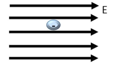
A positive charge moves in the direction of the field, while a negative charge moves opposite to the field.
The following experiment demonstrates the electric force on a test charge placed in an electric field and its motion. Click the play button to observe the direction of motion, which is the same as the force direction. You can change the field-generating charge's type and magnitude.
You can also determine the field direction by clicking the field icon.
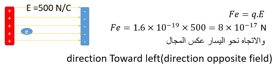
Determine the direction and magnitude of the force on an electron placed in the field in the following cases:
Non-Uniform Field
Uniform Field


\[F_e= .....................N \]
Click here to show solution
\[F_e= .....................N \]
Click here to show solution
3
A positively charged particle is placed in the field shown below. One of the following answers describes its motion:

Click here to show solution
Choose the correct answer
4
A ball of mass
\[m=5\;kg\] is dropped to the ground while carrying a charge of
\[q= 5\; µc\]. The uniform electric field vector that balances it is:

Click here to show solution
Choose the correct answer
>(Advanced) Dipole in an Electric Field
When a dipole is placed in a uniform field, each charge experiences an electric force, causing the dipole to rotate and produce a torque.

Considering the axis of rotation at one charge, the torque is:
\[ 𝜏 = r \cdot F \cdot \sin 𝜃 \]
\(r = d\) (distance between charges)
\(F = q E\) (force on one charge)
𝜃 is the angle between the arm and the force
Thus, the relationship is:
\[ 𝜏 = q \cdot d \cdot E \cdot \sin 𝜃 \]
\[ 𝜏 = p \cdot E \cdot \sin 𝜃 \]

Electric Flux

Electric Flux: The number of electric field lines passing perpendicularly through a surface area
Factors affecting electric flux:
Surface area, electric field intensity,
and the angle between the field and the normal to the surface
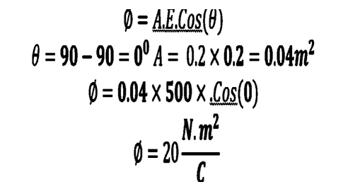
Electric flux is a scalar quantity given by the relation \[∅=A.E.Cos(𝜃) \] and is measured in units of \[\frac{N.m^2}{C}\]
5
One of the following units is equivalent to the unit of electric field intensity
Click here to show solution
Choose the correct answer
(0.2 m) square surface with side length
placed in a uniform electric field with intensity \[E=500\frac{N}{C}\] Calculate the flux in the following cases

Field makes 30° angle with surface
Field makes 30° angle with surface normal
\[...................\]
Click here to show solution
\[...................\]
Click here to show solution
Field perpendicular to surface
Field parallel to surface
\[...................\]
Click here to show solution
\[...................\]
Click here to show solution
Solved Example
Cube with side length
\[0..3m\] placed in a uniform electric field directed along the
\[X\] axis with intensity \[E=200\frac{N}{C}\] Calculate the flux through each face and the total flux

The cube has six faces: 1-front, 2-back, 3-top, 4-bottom, 5-right side, 6-left side
\[∅_1=∅_2=∅_3=∅_4=0.0\] because the field is parallel to the surface \[∅_5=A.E.Cos(𝜃)=(0.3 × 0.3)×200×Cos(0)=18\frac{N.m^2}{C} \] \[∅_6=A.E.Cos(𝜃)=(0.3 × 0.3)×200×Cos(180)=-18\frac{N.m^2}{C} \]Calculate the total flux through the cube \[∅_{net}=∅_1+∅_2+∅_3+∅_4+∅_5+∅_6=0+0+0+0+0+18-18=0\] Important result: If an object is placed in a uniform or non-uniform electric field, the net flux through the object is zero because the number of field lines entering equals those exiting


Gauss's Law (Deriving the law from Coulomb's Law)
Let there be a point charge generating an electric field around it, and we need to calculate the field at a point distance
\[r\]
We choose a Gaussian surface passing through the desired point where the field is constant on the Gaussian surface
Suppose we have a small area element
\[dA\] with electric field intensity
\[E\] passing through it
Then the flux is given by
\[d∅=dA.E.Cos(𝜃)\] \[∅=\oint{dA.E.Cos(0)}=E\oint{dA}=E.A=4𝜋r^2.\frac{q}{4𝜋ع_0r^2}\] \[∅=\oint{E.dA}=\frac{q}{ع_0}\]
This way we find the field without dealing with integration complexities
Results from Gauss's Law
The electric field inside an isolated conductor is always zero
When a conductor is placed in an electric field, its charges are affected by the field force, pushing negative charges opposite to the field and positive charges along the field
direction, creating an opposing field inside the conductor resulting in zero net field

Cavities inside conductors are protected from fields
When charging any conductor regardless of its shape, the charges are affected by a repulsive force and move away from each other, with the farthest point being the outer surface of the conductor. Thus, there are no charges inside the conductor and the field is zero.

Calculating the Field Due to an Infinitely Long Wire Using Gauss's Law
An infinitely long charged wire, find the field at a point at distance
\[r\] from the wire. We choose a Gaussian surface passing through the desired point where the field is constant on the Gaussian surface, and the cylinder satisfies this condition.
Apply Gauss's Law:

Note that the flux through the two bases of the cylinder is zero because the electric field is perpendicular to the outward normal of the surface.
We are left with the flux through the lateral surface of the cylinder, whose area is:
\[ 𝐴=2𝜋𝑟.𝐿\]
\[∅=\oint{\vec E.\vec {dA}}=\frac{q}{ε_0}\]
\[∅=\oint{dA.E.Cos(0)}=\frac{q}{ε_0}\] \[E.2𝜋𝑟.𝐿=\frac{λ.L}{ε_0}\]\[E=\frac{λ}{2𝜋𝑟.ε_0}\]
\[E=\frac{2k.λ}{r}\]
This way, we find the field without dealing with complex integrals.
6
An infinitely long wire has a field calculated at a point
\[0.3\;m\]
from the wire. The electric field value was:
( 2.5 × 10³N/C )
and the direction is shown in the figure. The number of electrons gained or lost per unit length is equivalent to:

Click here to show the solution
Choose the correct answer
Calculating the Field Due to an Infinite Non-Conducting Sheet
Using Gauss's Law
The sheet is charged with a density of
( 𝛿 c/m2 )
We choose a Gaussian surface passing through the desired point where the field is constant on the Gaussian surface, and the cylinder satisfies this condition.
In a non-conducting surface, the charges are distributed over the entire surface.
Apply Gauss's Law:

Note that the flux through the lateral surface of the cylinder is zero because the electric field is perpendicular to the outward normal of the surface.
We are left with the flux through the two bases of the cylinder.
\[∅=\oint{\vec E.\vec {dA}}=\frac{q}{ε_0}\]
\[∅=\oint{dA_1.E_1.Cos(0)}+\oint{dA_2.E_2.Cos(0)}+\oint{dA_3.E_3.Cos(90)}=\frac{q}{ε_0}\] \[E(A+A)=\frac{𝛿.A}{ε_0}\] \[E=\frac{𝛿}{2.ε_0}\]
Calculating the Field Due to an Infinite Conducting Sheet
Using Gauss's Law
The sheet is charged with a density of
( 𝛿 c/m2 )
We choose a Gaussian surface passing through the desired point where the field is constant on the Gaussian surface, and the cylinder satisfies this condition.
In a conducting surface, the charges are distributed on the outer surface.
Apply Gauss's Law:

Note that the flux through the lateral surface of the cylinder is zero because the electric field is perpendicular to the outward normal of the surface.
We are left with the flux through the top base of the cylinder.
\[∅=\oint{\vec E.\vec {dA}}=\frac{q}{ε_0}\]
\[∅=\oint{dA_1.E_1.Cos(0)}+\oint{dA_3.E_3.Cos(90)}=\frac{q}{ε_0}\] \[E.A=\frac{𝛿.A}{ε_0}\]
\[E=\frac{𝛿}{ε_0}\]
7
Two infinite conducting sheets are charged with equal density.
One of the following answers is correct.

Click here to show the solution
Choose the correct answer
Spherical Symmetry
Spherical Shell
Let's have a charged spherical shell of radius (R).
(r2) We want to calculate the field at a point outside the shell at distance from the center.
We choose a spherical surface passing through the desired point and calculate the flux through it.

Note the flux through the surface
\[∅=\oint{\vec E.\vec {dA}}=\frac{q}{ε_0}\]
\[∅=\oint{dA.E.Cos(0)}=\frac{q}{ε_0}\] \[E(4𝜋{r_2}^2)=\frac{q}{ε_0}\] \[E=\frac{q}{4𝜋{r_2}^2.ε_0}\]
If the point is inside the spherical shell at distance
\[r_1\]
There are no charges inside the shell \[∅=\oint{\vec E.\vec {dA}}=E.4𝜋{r_1}^2=0\]
Solid Non-Conducting Sphere
Let's have a solid non-conducting sphere of radius
\[R\]. We want to calculate the field at a point outside the sphere at distance from the center.
\[r\] We choose a spherical surface passing through the desired point and calculate the flux through it.

Note the flux through the surface
\[∅=\oint{\vec E.\vec {dA}}=\frac{q}{ε_0}\]
\[∅=\oint{dA.E.Cos(0)}=\frac{q_t}{ε_0}\] \[E(4𝜋r^2)=\frac{q_t}{ε_0}\]\[E=\frac{qt}{4𝜋r^2.ε_0}\] \[E=\frac{k.q_t}{r^2}\]
If the point is inside the solid sphere at distance
\[r_s\] part of the charges are inside the Gaussian surface \[∅=\oint{\vec E.\vec {dA}}=\frac{q_s}{ε_0}\] \[E(4𝜋{r_s}^2)=\frac{𝜌
.V_s}{ε_0}\]\[E(4𝜋{r_s}^2)=\frac{𝜌\frac{4}{3}𝜋{r_s}^3}{ε_0}\]
\[E=\frac{𝜌.r_s}{3ε_0}\]
We can use the second method to find the field inside the sphere
If the point is inside the solid sphere, part of the charges are inside the Gaussian surface \[∅=\oint{\vec E.\vec {dA}}=\frac{q_s}{ε_0}\]
\[\frac{q_s}{q_t}=\frac{𝜌.V_s}{𝜌.V_t}=\frac{\frac{4}{3}𝜋{r_s}^3}{\frac{4}{3}𝜋{R}^3}\]\[\frac{q_s}{q_t}=\frac{{r_s}^3}{R^3}\]
\[q_s=\frac{q_t{r_s}^3}{R^3}\]\[E(4𝜋{r_s}^2)=\frac{q_t{r_s}^3}{ε_0.R^3}\]\[E=\frac{q_t.r_s}{4𝜋.ε_0.R^3}\]
\[E=\frac{K.q_t.r_s}{R^3}\]
Calculating the Field Inside the Sphere \[E=\frac{K.q_t.r_1}{R^3}\]
Calculating the Field Outside the Sphere \[E=\frac{k.q_t}{r^2}\]
Calculating the Field Inside and Outside a Solid Sphere
We want to calculate the field at a point inside or outside the charged sphere.
We choose a spherical surface passing through the desired point and calculate the flux through it.
According to Gauss's Law
(Field * Gaussian surface area = Enclosed charge / Permittivity of free space )
If the point is inside the sphere
The Gaussian surface encloses part of the sphere's charge, but the charge is uniformly distributed. We follow the rule:
(Total charge of sphere / Gaussian sphere charge = Total volume of sphere / Gaussian sphere volume )
Finally, we obtain the relation mentioned at the beginning of the experiment.
If the point is outside the sphere
The Gaussian surface encloses the entire charge of the sphere.
According to Gauss's Law
(Field * Gaussian surface area = Enclosed charge / Permittivity of free space )
Finally, we obtain the relation mentioned at the beginning of the experiment.
Field inside the solid sphere
\[E=\frac{K.q_t.r}{R^3}\] \[E \propto {r}\] Field outside the solid sphere
\[E=\frac{k.q_t}{r^2}\]\[E \propto \frac{1}{{{r^2}}}\] where (r) is the distance from the center of the solid sphere.
If we plot the graph between the field and the distance from the center of the charged solid sphere, we get the following graph:

8
The relation between the field and the distance from the center of a charged solid non-conducting sphere was plotted, resulting in the following graph. The magnitude of the field at a point at distance
\[0.15\;m\] from the center is equivalent to:

Click here to show the solution
Choose the correct answer
🧮 Calculator
🗑️
✏️ قلم
Gauss's law and electric field |
Electric Field
It is a region surrounding a charge where the effects of electric force appear. It represents the resultant electric force acting on a charge divided by the charge.
The electric field is a vector quantity with magnitude and direction. \[\vec E=\frac{\vec F_e}{q}= \frac{\frac{K.Q.q}{r^2}}{q}=\frac{K.Q}{r^2}\]
There are two methods to determine direction:
First Method: Place a test charge at the point where direction needs to be determined. According to vector rules, the product of a number and a vector
If a positive test charge is placed, the field direction is the same as the force direction. If the test charge is negative, the field direction is opposite to the electric force direction.
Second Method: By drawing field lines for a positive charge and a negative charge
Field lines for a positive charge emerge from the charge
Field lines for a negative charge converge toward the charge
One of the following measurement units is equivalent to the electric field measurement unit
Click here to show solution method
Choose the correct answer
An electric field with intensity \[\vec E=3×10^2\frac {N}{C}\]
An electron is placed inside the field
The electric force acting on the electron equals
\[q_e=1.6 ×10^{-19}C\]
Choose the correct answer Click here to show solution method
Electric Field Mapping
Properties of Electric Field Lines
They are imaginary lines that emerge from positive charges and converge into negative charges
The density of field lines is directly proportional to the magnitude of the electric charge
The field direction at any point is tangent to the field line at that point
Electric field lines do not intersect
There are two types of electric fields
Uniform field: A field with constant magnitude and direction at all points, its lines are straight and parallel
Non-uniform field: A field with non-constant magnitude or direction or both
Electric Field Due to Point Charges
We previously found that the magnitude of the electric field for a point charge is given by the relation \[\vec E=\frac {\vec F_e}{q}=\frac {K.Q}{r^2}\]
Each point charge generates an electric field around it
If we have more than one charge, each charge generates a field with magnitude and direction
Solved Example
Two point charges
\[q_1 = -6 \;\;𝜇c \;\;\;\;\;\;\;\; q_2 = 4 \;\;𝜇c\]The first charge is placed at the origin
and the second charge is placed at position \[X=5\;\;cm\]Calculate the electric field at position \[X=8\;\;cm\]
Solution
\[E_1=K.\frac {q_1}{r_1^2}=8.99×10^9×\frac {6×10^{-6}}{0.08^2}=8.43×10^6\;\; N/c\] to the left
\[E_2=K.\frac {q_2}{r_2^2}=8.99×10^9×\frac {4×10^{-6}}{0.03^2}=39.95×10^6\;\; N/c\] to the right
\[E_{net}=E_2-E_1=39.95×10^6-8.43×10^6=31.52×10^6\]to the right
Solved Example
Two point charges
\[q_1 = -3 \;\;nc \;\;\;\;\;\;\;\; q_2 = 5 \;\;nc\]placed on triangle vertices as shown in the figure
Calculate the electric field at position
\[A\]
Non-Uniform Field Uniform Field \[F_e= .....................N \]
\[F_e= .....................N \]
A positively charged particle is placed in the field shown below. One of the following answers describes its motion:
Choose the correct answer A ball of mass
\[m=5\;kg\] is dropped to the ground while carrying a charge of
\[q= 5\; µc\]. The uniform electric field vector that balances it is:
Choose the correct answer When a dipole is placed in a uniform field, each charge experiences an electric force, causing the dipole to rotate and produce a torque.
Considering the axis of rotation at one charge, the torque is:
\[ 𝜏 = r \cdot F \cdot \sin 𝜃 \]
Electric Flux: The number of electric field lines passing perpendicularly through a surface area
Factors affecting electric flux:
Surface area, electric field intensity,
and the angle between the field and the normal to the surface
Electric flux is a scalar quantity given by the relation \[∅=A.E.Cos(𝜃) \] and is measured in units of \[\frac{N.m^2}{C}\]
One of the following units is equivalent to the unit of electric field intensity Choose the correct answer Field makes 30° angle with surface
Field makes 30° angle with surface normal
\[...................\]
\[...................\]
Field perpendicular to surface
Field parallel to surface
\[...................\]
\[...................\]
Let there be a point charge generating an electric field around it, and we need to calculate the field at a point distance
\[r\]
An infinitely long charged wire, find the field at a point at distance
\[r\] from the wire. We choose a Gaussian surface passing through the desired point where the field is constant on the Gaussian surface, and the cylinder satisfies this condition.
An infinitely long wire has a field calculated at a point
\[0.3\;m\] Choose the correct answer
Calculating the Field Due to an Infinite Non-Conducting Sheet
Using Gauss's Law
The sheet is charged with a density of
Two infinite conducting sheets are charged with equal density.
One of the following answers is correct.
Choose the correct answer
Let's have a charged spherical shell of radius (R).
Let's have a solid non-conducting sphere of radius
\[R\]. We want to calculate the field at a point outside the sphere at distance from the center.
\[r\] We choose a spherical surface passing through the desired point and calculate the flux through it.
The relation between the field and the distance from the center of a charged solid non-conducting sphere was plotted, resulting in the following graph. The magnitude of the field at a point at distance
\[0.15\;m\] from the center is equivalent to:
Choose the correct answer
Solution
\[E_1=K.\frac {q_1}{r_1^2}=8.99×10^9×\frac {3×10^{-9}}{0.03^2}=29.9×10^3\;\; N/c\] to the left
\[E_2=K.\frac {q_2}{r_2^2}=8.99×10^9×\frac {5×10^{-9}}{0.04^2}=28.1×10^3\;\; N/c\] downward
\[E_{net}=\sqrt {E_2^2+E_1^2}=\sqrt {(29.9×10^3)^2+(28.1×10^3)^2}=41.1×10^3\;\;N/C\]Direction \[\theta=tan^{-1}\frac{E_2}{E_1}=tan^{-1}(\frac{28.1×10^3}{29.9×10^3})=43.2.2^0\]
(Self-Reading) Electric Field of a Dipole
Dipole: A charged object with two equal and opposite charges.
The field due to each charge is calculated, and vector addition is performed according to vector rules.
Solved Example
Calculate the electric field of a dipole along its axis at a point a distance
(X) from the center of the dipole.
The point is subject to two fields: from the positive charge
\[E_1=\frac{1}{4𝜋𝜀_0}\frac{q}{(X-\frac{1}{2}d)^2}\] (direction to the right)
and from the negative charge
\[E_2=\frac{1}{4𝜋𝜀_0}\frac{q}{(X+\frac{1}{2}d)^2}\] (direction to the left)
The resultant field is \[E_{net}=E_1-E_2\]
\[E_1>E_2\]
\[E_{net}=\frac{1}{4𝜋𝜀_0}\frac{q}{(X-\frac{1}{2}d)^2}-\frac{1}{4𝜋𝜀_0}\frac{q}{(X+\frac{1}{2}d)^2}\]
Direction to the right
Factoring out \[\frac{q}{4𝜋𝜀_0X^2}\]
The equation becomes \[E_{net}=\frac{q}{4𝜋𝜀_0X^2}\left[\frac{1}{(1-\frac{d}{2X})^2}-\frac{1}{(1+\frac{d}{2X})^2}\right]\] Combining denominators \[E_{net}=\frac{q}{4𝜋𝜀_0X^2}\left[\frac{(1+\frac{d}{2X})^2-(1-\frac{d}{2X})^2}{(1-\frac{d}{2X})^2(1+\frac{d}{2X})^2}\right]\]
\[E_{net}=\frac{q}{4𝜋𝜀_0X^2}\left[\frac{(1+\frac{d}{X}+\frac{d^2}{4X^2})-(1-\frac{d}{X}+\frac{d^2}{4X^2})}{(1-\frac{d}{2X})^2(1+\frac{d}{2X})^2}\right]\]
\[E_{net}=\frac{q}{4𝜋𝜀_0X^2}\left[\frac{(1+\frac{d}{X}+\frac{d^2}{4X^2}-1+\frac{d}{X}-\frac{d^2}{4X^2})}{(1-\frac{d}{2X})^2(1+\frac{d}{2X})^2}\right]\]
If \(X \gg d\)
\[\frac{d}{2X} \approx 0\]\[E_{net}=\frac{2dq}{4𝜋𝜀_0X^3}=\frac{dq}{2𝜋𝜀_0X^3}=\frac{2kdq}{X^3}\]
\[P=q.d\] is called the dipole moment, a vector quantity with direction from the negative to the positive charge, opposite to the electric field.
Solved Example
Calculate the electric field of a dipole at a point on the perpendicular bisector, a distance
(y) from the center of the dipole.
The point is subject to two fields \[E_1,E_2\]. When resolving each field into components, symmetry shows that
\[𝐸_{1y} = {𝐸_2y}\] and their resultant is zero.
From the figure \[r=\sqrt{(\frac{d}{2})^2+y^2}, \cos 𝜃= \frac{\frac{d}{2}}{r}\]
\[E_{1X}=E_1 \cos 𝜃=\frac{k q}{r^2} \cdot \frac{\frac{d}{2}}{r}=\frac{k q}{(\frac{d}{2})^2+y^2} \cdot \frac{\frac{d}{2}}{\sqrt{(\frac{d}{2})^2+y^2}}\]
\[𝐸_{1x} =\frac{k q d}{2[{(\frac{d}{2})^2+y^2}]^{3/2}}\]
\[E_{2X}=E_2 \cos 𝜃=\frac{k q}{r^2} \cdot \frac{\frac{d}{2}}{r}=\frac{k q}{(\frac{d}{2})^2+y^2} \cdot \frac{\frac{d}{2}}{\sqrt{(\frac{d}{2})^2+y^2}}\]
\[𝐸_{2x} =\frac{k q d}{2[{(\frac{d}{2})^2+y^2}]^{3/2}}\]
\[E_{net}=𝐸_{1x}+𝐸_{2x}=\frac{k q d}{2[{(\frac{d}{2})^2+y^2}]^{3/2}}+\frac{k q d}{2[{(\frac{d}{2})^2+y^2}]^{3/2}}\]
\[E_{net}= -\frac{k q d}{[{(\frac{d}{2})^2+y^2}]^{3/2}}\]
The negative sign indicates the direction is along the negative horizontal axis.
If \(y \gg d\)
\[\frac{d}{2} \approx 0\]
\[E_{net}= -\frac{k q d}{y^3} \]
General Charge Distributions
For a very large number of charges, calculating the resultant field using the previous method is impractical. Instead, integration is used, provided the charges are uniformly distributed.
Take a small part of the object's charge
\[dq\]
calculate its field, then integrate over the entire object.
The problem arises if the charge is distributed along a line, over a surface, or within a volume.
Along a line:
\[𝑑𝑞=λ𝑑𝑥\]
Over a surface:
\[𝑑𝑞=σ𝑑A\]
Within a volume:
\[𝑑𝑞=𝜌𝑑V\]
(Advanced) Solved Example
A finite-length wire is uniformly charged as shown below. Calculate the magnitude and direction of the field at a point along the perpendicular bisector of the wire.
Take a small charge
\[dq\] and calculate its field, then integrate over the entire wire.
Considering half the wire, symmetry shows that
\[E_1X=E_2X\]
They cancel each other out, so the resultant is zero.
The vertical components from each half are equal in magnitude and direction.
\[ d𝐸_1Y =d 𝐸_1 \cos 𝜃 , d𝐸_2Y =d 𝐸_2 \cos 𝜃\]
To calculate the field, compute it for half the wire and double the result.
.
From the figure \[r=\sqrt{X^2+Y^2}, \cos 𝜃= \frac{Y}{r}\]
\[E=2\int_{0}^{a}{dE_Y}=2\int_{0}^{a}{k\frac{dq}{r^2}\cos 𝜃}=2k\int_{0}^{a}{\frac{λ𝑑𝑥}{r^2}\frac{Y}{r}}\]
\[E=2kλY\int_{0}^{a}{\frac{𝑑𝑥}{(X^2+Y^2)^{3/2}}}\]
The integral is solved using standard tables.
\[\int_{0}^{a}{\frac{𝑑𝑥}{(X^2+Y^2)^{3/2}}}=\left|\frac{1}{Y^2}\frac{X}{\sqrt{X^2+Y^2}}\right|_{0}^{a}=\frac{1}{Y^2}\frac{a}{\sqrt{a^2+Y^2}}\]
\[E=2kλY\frac{1}{Y^2}\frac{a}{\sqrt{a^2+Y^2}}\]
The field due to a finite-length wire is:
\[E=2kλ\frac{1}{Y}\frac{a}{\sqrt{a^2+Y^2}}\] where \(a\) is half the wire's length.

For an infinitely long wire, a→∞\[\frac{a}{\sqrt{a^2+Y^2}}→1\]
\[E=\frac{2kλ}{y}\]
Force Due to Electric Field
If a charge is placed in an electric field, it experiences an electric force:
\[\vec F_e=q \vec E\]
A positive charge moves in the direction of the field, while a negative charge moves opposite to the field.
The following experiment demonstrates the electric force on a test charge placed in an electric field and its motion. Click the play button to observe the direction of motion, which is the same as the force direction. You can change the field-generating charge's type and magnitude.
You can also determine the field direction by clicking the field icon.
Determine the direction and magnitude of the force on an electron placed in the field in the following cases:
 Click here to show solution
 Click here to show solution
 Click here to show solution
 Click here to show solution
>(Advanced) Dipole in an Electric Field
\(r = d\) (distance between charges)
\(F = q E\) (force on one charge)
𝜃 is the angle between the arm and the force
Thus, the relationship is:
\[ 𝜏 = q \cdot d \cdot E \cdot \sin 𝜃 \]
\[ 𝜏 = p \cdot E \cdot \sin 𝜃 \]
Electric Flux
Click here to show solution
placed in a uniform electric field with intensity \[E=500\frac{N}{C}\] Calculate the flux in the following cases
 Click here to show solution
 Click here to show solution
 Click here to show solution
 Click here to show solution
The cube has six faces: 1-front, 2-back, 3-top, 4-bottom, 5-right side, 6-left side
\[∅_1=∅_2=∅_3=∅_4=0.0\] because the field is parallel to the surface \[∅_5=A.E.Cos(𝜃)=(0.3 × 0.3)×200×Cos(0)=18\frac{N.m^2}{C} \] \[∅_6=A.E.Cos(𝜃)=(0.3 × 0.3)×200×Cos(180)=-18\frac{N.m^2}{C} \]Calculate the total flux through the cube \[∅_{net}=∅_1+∅_2+∅_3+∅_4+∅_5+∅_6=0+0+0+0+0+18-18=0\] Important result: If an object is placed in a uniform or non-uniform electric field, the net flux through the object is zero because the number of field lines entering equals those exiting
We choose a Gaussian surface passing through the desired point where the field is constant on the Gaussian surface
Suppose we have a small area element
\[dA\] with electric field intensity
\[E\] passing through it
Then the flux is given by
\[d∅=dA.E.Cos(𝜃)\] \[∅=\oint{dA.E.Cos(0)}=E\oint{dA}=E.A=4𝜋r^2.\frac{q}{4𝜋ع_0r^2}\] \[∅=\oint{E.dA}=\frac{q}{ع_0}\]
This way we find the field without dealing with integration complexities
Results from Gauss's Law
The electric field inside an isolated conductor is always zero
When a conductor is placed in an electric field, its charges are affected by the field force, pushing negative charges opposite to the field and positive charges along the field
direction, creating an opposing field inside the conductor resulting in zero net field
Cavities inside conductors are protected from fields
When charging any conductor regardless of its shape, the charges are affected by a repulsive force and move away from each other, with the farthest point being the outer surface of the conductor. Thus, there are no charges inside the conductor and the field is zero.
Calculating the Field Due to an Infinitely Long Wire Using Gauss's Law
Apply Gauss's Law:
Note that the flux through the two bases of the cylinder is zero because the electric field is perpendicular to the outward normal of the surface.
We are left with the flux through the lateral surface of the cylinder, whose area is:
\[ 𝐴=2𝜋𝑟.𝐿\]
\[∅=\oint{\vec E.\vec {dA}}=\frac{q}{ε_0}\]
\[∅=\oint{dA.E.Cos(0)}=\frac{q}{ε_0}\] \[E.2𝜋𝑟.𝐿=\frac{λ.L}{ε_0}\]\[E=\frac{λ}{2𝜋𝑟.ε_0}\]
\[E=\frac{2k.λ}{r}\]
This way, we find the field without dealing with complex integrals.
from the wire. The electric field value was:
( 2.5 × 10³N/C )
and the direction is shown in the figure. The number of electrons gained or lost per unit length is equivalent to:
Click here to show the solution
( 𝛿 c/m2 )
We choose a Gaussian surface passing through the desired point where the field is constant on the Gaussian surface, and the cylinder satisfies this condition.
In a non-conducting surface, the charges are distributed over the entire surface.
Apply Gauss's Law:
Note that the flux through the lateral surface of the cylinder is zero because the electric field is perpendicular to the outward normal of the surface.
We are left with the flux through the two bases of the cylinder.
\[∅=\oint{\vec E.\vec {dA}}=\frac{q}{ε_0}\]
\[∅=\oint{dA_1.E_1.Cos(0)}+\oint{dA_2.E_2.Cos(0)}+\oint{dA_3.E_3.Cos(90)}=\frac{q}{ε_0}\] \[E(A+A)=\frac{𝛿.A}{ε_0}\] \[E=\frac{𝛿}{2.ε_0}\]
Calculating the Field Due to an Infinite Conducting Sheet
Using Gauss's Law
The sheet is charged with a density of
( 𝛿 c/m2 )
We choose a Gaussian surface passing through the desired point where the field is constant on the Gaussian surface, and the cylinder satisfies this condition.
In a conducting surface, the charges are distributed on the outer surface.
Apply Gauss's Law:
Note that the flux through the lateral surface of the cylinder is zero because the electric field is perpendicular to the outward normal of the surface.
We are left with the flux through the top base of the cylinder.
\[∅=\oint{\vec E.\vec {dA}}=\frac{q}{ε_0}\]
\[∅=\oint{dA_1.E_1.Cos(0)}+\oint{dA_3.E_3.Cos(90)}=\frac{q}{ε_0}\] \[E.A=\frac{𝛿.A}{ε_0}\]
\[E=\frac{𝛿}{ε_0}\]
Click here to show the solution
Spherical Symmetry
Spherical Shell
(r2) We want to calculate the field at a point outside the shell at distance from the center.
We choose a spherical surface passing through the desired point and calculate the flux through it.
Note the flux through the surface
\[∅=\oint{\vec E.\vec {dA}}=\frac{q}{ε_0}\]
\[∅=\oint{dA.E.Cos(0)}=\frac{q}{ε_0}\] \[E(4𝜋{r_2}^2)=\frac{q}{ε_0}\] \[E=\frac{q}{4𝜋{r_2}^2.ε_0}\]
If the point is inside the spherical shell at distance
\[r_1\]
There are no charges inside the shell \[∅=\oint{\vec E.\vec {dA}}=E.4𝜋{r_1}^2=0\]
Solid Non-Conducting Sphere
Note the flux through the surface
\[∅=\oint{\vec E.\vec {dA}}=\frac{q}{ε_0}\]
\[∅=\oint{dA.E.Cos(0)}=\frac{q_t}{ε_0}\] \[E(4𝜋r^2)=\frac{q_t}{ε_0}\]\[E=\frac{qt}{4𝜋r^2.ε_0}\] \[E=\frac{k.q_t}{r^2}\]
If the point is inside the solid sphere at distance
\[r_s\] part of the charges are inside the Gaussian surface \[∅=\oint{\vec E.\vec {dA}}=\frac{q_s}{ε_0}\] \[E(4𝜋{r_s}^2)=\frac{𝜌
.V_s}{ε_0}\]\[E(4𝜋{r_s}^2)=\frac{𝜌\frac{4}{3}𝜋{r_s}^3}{ε_0}\]
\[E=\frac{𝜌.r_s}{3ε_0}\]
We can use the second method to find the field inside the sphere
If the point is inside the solid sphere, part of the charges are inside the Gaussian surface \[∅=\oint{\vec E.\vec {dA}}=\frac{q_s}{ε_0}\]
\[\frac{q_s}{q_t}=\frac{𝜌.V_s}{𝜌.V_t}=\frac{\frac{4}{3}𝜋{r_s}^3}{\frac{4}{3}𝜋{R}^3}\]\[\frac{q_s}{q_t}=\frac{{r_s}^3}{R^3}\]
\[q_s=\frac{q_t{r_s}^3}{R^3}\]\[E(4𝜋{r_s}^2)=\frac{q_t{r_s}^3}{ε_0.R^3}\]\[E=\frac{q_t.r_s}{4𝜋.ε_0.R^3}\]
\[E=\frac{K.q_t.r_s}{R^3}\]
Calculating the Field Inside the Sphere \[E=\frac{K.q_t.r_1}{R^3}\]
Calculating the Field Outside the Sphere \[E=\frac{k.q_t}{r^2}\]
Calculating the Field Inside and Outside a Solid Sphere
We want to calculate the field at a point inside or outside the charged sphere.
We choose a spherical surface passing through the desired point and calculate the flux through it.
According to Gauss's Law
(Field * Gaussian surface area = Enclosed charge / Permittivity of free space )
If the point is inside the sphere
The Gaussian surface encloses part of the sphere's charge, but the charge is uniformly distributed. We follow the rule:
(Total charge of sphere / Gaussian sphere charge = Total volume of sphere / Gaussian sphere volume )
Finally, we obtain the relation mentioned at the beginning of the experiment.
If the point is outside the sphere
The Gaussian surface encloses the entire charge of the sphere.
According to Gauss's Law
(Field * Gaussian surface area = Enclosed charge / Permittivity of free space )
Finally, we obtain the relation mentioned at the beginning of the experiment.
Field inside the solid sphere
\[E=\frac{K.q_t.r}{R^3}\] \[E \propto {r}\] Field outside the solid sphere
\[E=\frac{k.q_t}{r^2}\]\[E \propto \frac{1}{{{r^2}}}\] where (r) is the distance from the center of the solid sphere.
If we plot the graph between the field and the distance from the center of the charged solid sphere, we get the following graph:
Click here to show the solution
No comments:
Post a Comment